pointfree | Ulisses Costa Blog

More Hylomorphisms in Haskell

9 04 2009

If you lost yourself in this post, I advise you to start in catamorphisms, then anamorphisms and then hylomorphisms.

Like I said before (in those posts) when you write an hylomorphism over a particular data type, that means just that the intermediate structure is that data type.

In fact that data will never be stored into that intermediate type $C$ or $D$ . Because we glue the ana and cata together into a single recursive pattern. $A$ and $E$ could be some data type your function need. With this post I will try to show you more hylomorphisms over some different data types to show you the power of this field.

Leaf Tree’s

The data type that we going to discuss here is the $LTree$ . In Haskell we can represent $LTree$ as:

data LTree a = Leaf a | Fork (LTree a, LTree a)

Is just like a binary tree, but the information is just in the leaf’s. Even more: a leaf tree is a tree that only have leaf’s, no information on the nodes. This is an example of a leaf tree:

To represent all the hylomorphisms over $Ltree$ we draw the following diagram:

The example I’m going to give is making the fibonacci function using a hylomorphism over this data type. If you remember the method I used before, I’m going to start by the anamorphism $[(h)]$ . Before that I’m going to specify the strategy to define factorial. I’m going to use the diagram’s again, remember that type $1$ is equivalent to Haskell $( )$ :

As you can see I’m going to use $Ltree~1$ as my intermediate structure, and I’ve already define the names of my gen functions $add$ to the catamorphism and $fibd$ to the anamorphism. The strategy I prefer, is do all the hard work in the anamorphism, so here the gen $fibd$ for the anamorphism is:

fibd n | n < 2     = i1   ()
       | otherwise = i2   (n-1,n-2)

This function combined with the anamorphism, going to generate leaf tree’s with $n$ leaf’s, being $n$ the result of that fib.

Then we just have to write the gen $add$ for the catamorphism. This function (combined with the catamorphism) counts the number of leafs that a leaf tree have.

add = either (const 1) plus
    where plus = uncurry (+)

The final function, the fibonacci function is the hylomorphism of those two defined before:

fib =  hyloLTree add fibd

Here is all the auxiliary functions you need to run this example:

inLTree = either Leaf Fork

outLTree :: LTree a -> Either a (LTree a,LTree a)
outLTree (Leaf a)     = i1   a
outLTree (Fork (t1,t2)) = i2    (t1,t2)

cataLTree a = a . (recLTree (cataLTree a)) . outLTree

anaLTree f = inLTree . (recLTree (anaLTree f) ) . f

hyloLTree a c = cataLTree a . anaLTree c

baseLTree g f = g -|- (f >< f)

recLTree f = baseLTree id f

Lists

The lists that I’m going to talk here, are the Haskell lists, wired into the compiler, but is a definition exist, it will be:

data [a] = [ ] | a : [a]

So, our diagram to represent the hylomorphism over this data type is:

The function I’m going to define as a hylomorphism is the factorial function. So, we know that our domain and co-domain is $Integers$ , so now we can make a more specific diagram to represent our solution:

As you can see I’m going to use $[Integer]$ to represent my intermediate data, and I’ve already define the names of my gen functions $mul$ to the catamorphism and $nats$ to the anamorphism. Another time, that I do all the work with the anamorphism, letting the catamorphism with little things to do (just multiply). I’m start to show you the catamorphism first:

mul = either (const 1) mul'
    where mul' = uncurry (*)

As you can see the only thing it does is multiply all the elements of a list, and multiply by 1 when reach the $[]$ empty list.

In the other side, the anamorphism is generating a list of all the elements, starting in $n$ (the element we want to calculate the factorial) until 1.

nats = (id -|- (split succ id)) . outNat

And finally we combine this together with our hylo, that defines the factorial function:

fac = hylo mul nats

Here is all the code you need to run this example:

inl = either (const []) (uncurry (:))

out []    = i1 ()
out (a:x) = i2(a,x)

cata g   = g . rec (cata g) . out   

ana h    = inl . (rec (ana h) ) . h

hylo g h = cata g . ana h

rec f    = id -|- id >< f

Binary Tree’s

Here, I’m going to show you the hanoi problem solved with one hylomorphism, first let’s take a look at the $Btree$ structure:

data BTree a = Empty | Node(a, (BTree a, BTree a))

So, our generic diagram representing one hylomorphism over $BTree$ is:

There is a well-known inductive solution to the problem given by the pseudocode below. In this solution we make use of the fact that the given problem is symmetrical with respect to all three poles. Thus it is undesirable to name the individual poles. Instead we visualize the poles as being arranged in a circle; the problem is to move the tower of disks from one pole to the next pole in a speciﬁed direction around the circle. The code deﬁnes $H_n.d$ to be a sequence of pairs $(k, d)$ where n is the number of disks, $k$ is a disk number and $d$ are directions. Disks are numbered from $0$ onwards, disk $0$ being the smallest. Directions are boolean values, $true$ representing a clockwise movement and $false$ an anti-clockwise movement. The pair $(k, d)$ means move the disk numbered $k$ from its current position in the direction $d$ .

excerpt from R. Backhouse, M. Fokkinga / Information Processing Letters 77 (2001) 71–76

So, here, I will have a diagram like that, $b$ type stands for $Bool$ and $i$ type for $Integer$ :

I’m going to show all the solution here, because the description of the problem is in this quote, and in the paper:

hanoi = hyloBTree f h

f = either (const []) join
    where join(x,(l,r))=l++[x]++r

h(d,0) = Left ()
h(d,n+1) = Right ((n,d),((not d,n),(not d,n)))

And here it is, all the code you need to run this example:

inBTree :: Either () (b,(BTree b,BTree b)) -> BTree b
inBTree = either (const Empty) Node

outBTree :: BTree a -> Either () (a,(BTree a,BTree a))
outBTree Empty              = Left ()
outBTree (Node (a,(t1,t2))) = Right(a,(t1,t2))

baseBTree f g = id -|- (f >< g))

cataBTree g = g . (recBTree (cataBTree g)) . outBTree

anaBTree g = inBTree . (recBTree (anaBTree g) ) . g

hyloBTree h g = cataBTree h . anaBTree g

recBTree f = baseBTree id f

Outroduction

Maybe in the future I will talk more about that subject.

Comments : 3 Comments »
Tags: anamorphism, catamorphism, code, English, functions, hacking, haskell, hylomorphism, mathematics, mp1, pointfree, programming, recursion, types
Categories : Uncategorized

Hylomorphisms in Haskell

9 04 2009

If you miss something in this post, I suggest you to start in Catamorphisms and Anamorphisms.

A Hylomorphism is just the composition of one catamorphism and then one anamorphism.
$hylo~f~h~=~cata~f~\circ~ana~h$ , replacing that by the proper notation we have: $[|f,h|]~=~(|f|)~\circ~[(h)]$

In this post I will use the structure of a binary tree:

data BTree a = Empty | Node(a, (BTree a, BTree a))

I will use the tuples to don’t have to write uncurry’s. As I will show you, when we say that we are making a hylomorphism on a particular data type $T$ , what we are trying to say is that the intermediate structure of our combination of catamorphism and anamorphism is that data type $T$ . This is the structure throw our morphism will communicate with each other.

Anamorphism

So, here I will solve the Quicksort algorithm with a hylomorphism over $BTree$ .

The intermediate structure being a $BTree$ doesn’t mean that my function will receive $BTree$ . My $qSort$ function works over lists. So the first thing to do, is draw the respective anamorphism from $[a]$ to $BTree~a$ :

My strategy here is to do all the work in the anamorphism, so, I need a function $h$ with type:
$h : [a] \rightarrow 1 + a \times [a] \times [a]$ , or in Haskell $h :: [a] \rightarrow Either () (a, ([a], [a]))$

That function is $qsep$ :

qsep :: [a] -> Either () (a, ([a], [a]))
qsep []    = Left ()
qsep (h:t) = Right (h,(s,l))
    where (s,l) = part (<h) t

part:: (a -> Bool) -> [a] -> ([a], [a])
part p []                = ([],[])
part p (h:t) | p h       = let (s,l) = part p t in (h:s,l)
             | otherwise = let (s,l) = part p t in (s,h:l)

This code is very simple, in $qsep$ I chose a pivotal element (first one), and filter the bigger to one side, and the other ones to the other, just like the algorithm. The function that do all that job is $part$ , it process all the list finding the elements that satisfy the condition $p$ , to put them in the left side of the tuple, and the others into the right side.

This function by it self don’t do almost anything, it is only a simple part of the algorithm.

Catamorphism

Next step is to see the diagram for catamorphisms from $BTree~a$ to $[a]$ :

As I said before, the heavy duty is on the side of the anamorphism, so here, the catamorphism will be very very simple. In fact it is.

inord :: Either a (a, ([a], [a])) -> [a]
inord = either (const []) join
    where join(x,(l,r))=l++[x]++r

That right! The only thing that the catamorphism do is a inorder passage over the structures $a + a \times [a] \times [a]$ , which is very simple, as as shown by the code.

Hylomorphism

The first thing is to draw the diagram, now for the hylomorphism, the composition of the cata with the ana:

Once having made the two most important parts of the function (the ana and cata), the hylo is very simple to do. You just have to make a function $hyloBTree$ :

hyloBTree h g = cataBTree h . anaBTree g

And our function $qSort$ bacame:

qSort :: Ord a => [a] -> [a]
qSort = hyloBTree inord qsep

And that’s it, now I’m going to show you the all code that you need to put all the things together and working.

inBTree :: Either () (b,(BTree b,BTree b)) -> BTree b
inBTree = either (const Empty) Node

outBTree :: BTree a -> Either () (a,(BTree a,BTree a))
outBTree Empty              = Left ()
outBTree (Node (a,(t1,t2))) = Right(a,(t1,t2))

baseBTree f g = id -|- (f >< g))

cataBTree g = g . (recBTree (cataBTree g)) . outBTree

anaBTree g = inBTree . (recBTree (anaBTree g) ) . g

hyloBTree h g = cataBTree h . anaBTree g

recBTree f = baseBTree id f

Outroduction

If you need more explanations feel free to contact me.

Comments : 3 Comments »
Tags: anamorphism, catamorphism, code, English, functions, haskell, hylomorphism, mathematics, pointfree, programming, recursion, Theoretical fundations, theory
Categories : Uncategorized

Anamorphisms in Haskell

8 04 2009

First I would like to introduce the notation that I use here. The pointfree notation is good to see a program (functions) data flow and as composition of functions, combination of functions, if you prefer. This style is characterized by not using variables in declaration of functions. Haskell allow us to implement that notation natively. The dual of the pointfree notation is the pointwise one.

A simple example of a function in pointwise style:

f n = (n+2)*10 -- pointwise

The dual in pointfree would be:

f = (*10) . (+2) -- pointfree

Clarifications

First of all to define a function, for example $f$ , i can say:

, or .

I will assume that you are familiarized with infix notation, $either$ , and composition $(\circ)$ functions.

Types

For this post I need to explain the data type we will going to use. In Haskell we define it by:

data Tree a = Node a [Tree a]

Let’s create the same, but more convenient. Consider the following isomorphic type for $Tree$ :

data Tree a = Node (a, [Tree a])

We could see $Node$ as a the following function:

Node :: (a, [Tree a]) -> Tree a

So typologically we have $(a, [Tree~a])$ . We use $(\times)$ to define that two things occurs in parallel, like tuples do, so we can redefine it: $(a \times~[Tree~a])$

Now we can say that $(Tree~a)$ is isomorphic to $(a \times~[Tree~a])$ .
This is something to say that $(Tree~a)$ and $(a \times~[Tree~a])$ keep the same information without any change. We represent that formally as: $(Tree~a) \cong~(a \times~[Tree~a])$ .

Anamorphisms

Let $A$ , $B$ , $C$ , $D$ be Inductive data types (sets) and $in$ , $ana$ , $rec$ functions.

$ana(h_{Tree})$ is the anamorphism of $h$ if the diagram commute.

We use the notation $rec_{Tree}$ to say that function $rec$ in not generic, but only works for data $Tree$ . The same happens with $in$ and $ana$ . We will write $ana(h)_{Tree}$ using the composition of $in$ , $ana$ and $rec$ functions. That way we are breaking our problem in small ones. So, in the end we will have the following definition for $ana(h)_{Tree}$ :

$ana(h)_{Tree} = in_{Tree} \circ rec_{Tree} \circ h$

The function that we want is $ana(h)$ , and that function is over $(Tree~a)$ so we have:

ana :: (A -> B) -> A -> Tree c

Type $C$ is $(Tree~c)$ . Maybe this isn’t clear yet, let’s start with function $in$

function in

The function $in_{Tree}$ is responsible to create the isomorphism between $(Tree~a)$ and $(a \times~[Tree~a])$ , so the code could be something like this:

inTree :: Tree a -> (a, [Tree a])
inTree    = Node

In Haskell we represent the type $(\times)$ as $(,)$ . So, type $D$ is $(a \times~[Tree~a])$ . So by now, we already know the following unifications $C \sim Tree~c$ and $D \sim c \times~[Tree~c]$ . So now our graphic is:

function $h$

The function $h$ is also known as *gen*, here is where we said the step that pattern do. This is the only function we need to take care, if this function is good, our problem is solved. Now image that our problem is:

Suppose that the pair of positive integers (v, p) denotes the number of red balls (v) and black (p) that is inside a bag, the balls which are taking randomly, successively, until the bag is empty.

This is the point-wise version of the function we want to convert to pointfree using anamorphisms. This function represent as a tree, all possible states of the bag over these experiences.

state :: (Int,Int) -> Tree (Int,Int)
state(0,0) = Node (0,0) []
state(v,0) = Node (v,0) [state(v-1,0)]
state(0,p) = Node (0,p) [state(0,p-1)]
state(v,p) = Node (v,p) [state(v-1,p),state(v,p-1)]

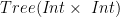
If we want that “latex state$ became an anamorphism, we have to say that our type $A$ unify ( $\sim$ ) with $Int \times~Int$ , and $Tree~c$ became more restrict, and unify with $Tree (Int \times~Int)$ . A consequence of changing the co-domain of $in_{Tree}$ is changing the domain of it to $(Int \times~Int) \times~[Tree (Int \times~Int)]$ . We represent $ana(h)$ as $[( h )]$ . Now we can be more specific with our graphic:

function rec

Here we have to get a function $rec$ that co-domain is $(Int \times~Int) \times~[Tree~(Int \times~Int)]$ . Probably the best is to pass the first part of the tuple (part with type $(Int \times~Int)$ ) and the rest (part with type $[Tree~(Int \times~Int)]$ ) is just a $map$ of the function $[(h)]_{Tree}$ . So, now our graphic is:

As you can see, the second part of the co-domain of $h$ is the type of function $map~[(h)]_{Tree}$ :

$map~[(h)]_{Tree}~:~[(Int \times~Int)] \rightarrow~[Tree(Int \times~Int)]$

So our final graphic became:

Now, we just have to define the function $h$ and apply them to our anamorphism of $Tree$ .

h :: (Int, Int) -> ( (Int, Int), [ (Int, Int) ] )
h(0,0) = ( (0,0), [] )
h(v,0) = ( (v,0), [ (v-1,0) ] )
h(0,p) = ( (0,p) [ (0,p-1) ] )
h(v,p) = ( (v,p), [ (v-1,p), (v,p-1) ] )

And this is it! Now we can say that:
$state \equiv~ana_{Tree}$ where $ana(h)_{Tree} = in_{Tree} \circ~id~><~map~ana(h)_{Tree} \circ h$

Outroduction

Here is all the code you need to run this example in Haskell:

module AnamorphismExample where

infix 5 ><

i1 = Left
i2 = Right
p1 = fst
p2 = snd

data Tree a = Node (a, [Tree a]) deriving Show

split :: (a -> b) -> (a -> c) -> a -> (b,c)
split f g x = (f x, g x)

(><) :: (a -> b) -> (c -> d) -> (a,c) -> (b,d)
f >< g = split (f . p1) (g . p2)

inTree :: (a, [Tree a]) -> Tree a
inTree = Node

anaTree h = inTree . (id >< map (anaTree h)) . h

-- our function
h_gen :: (Int, Int) -> ( (Int, Int), [ (Int, Int) ] )
h_gen(0,0) = ( (0,0), [] )
h_gen(v,0) = ( (v,0), [ (v-1,0) ] )
h_gen(0,p) = ( (0,p) , [ (0,p-1) ] )
h_gen(v,p) = ( (v,p), [ (v-1,p), (v,p-1) ] )

state = anaTree h_gen

Pass a year since I promised this post. The next will be on hylomorphisms I promise not take too that much.

Comments : 6 Comments »
Tags: anamorphism, code, English, functions, haskell, mathematics, mp1, pointfree, programming, recursion, Theoretical fundations
Categories : Uncategorized

Type inference

30 07 2008

Intro

The type inference is the ability to a programming language deduct the data types of all functions of a program. It is a feature present in many strongly typed languages, such as Haskell. Where is not mandatory write the signature of the functions. What is great because it increases the production of code, and security because if the inference algorithm fail means that we have an error of types in our code, all this in compilation time.

As I said in previous post, one of the upgrades of Pointfree calculator is the type inference. After reading some scientific articles about Damas-Milner algorithm, also known as W algorithm, I began to imagine a way to implement this in Java, which is the mother language of Pointfree calculator. I started to do some sketches on paper and, after talking with professor José Nuno Oliveira, I realize that the algorithm isn’t that hard.

Remainings

Definition of (either in Haskell):

NOTE: in types means Either in Haskell

Definition of :

Type signature of Left and Right:

Talking same language

I will use a different notation to represent the domain and codomain of functions in order to help the explanation of the algorithm.

For function we have the type:

I will write that as:

Remember the definition of , we receive two functions, f and g. Because the notation is in pointfree, we represent also de domain and codomain of function in front of that, like we do for f and g.
In fact the type of is represented as:

I will also use the symbol , to say that type a unify with type b, that means, informally, that .

Let’s infer!

I will explain the algorithm to infer the type of function f:

The first step of the algorithm is attribute to all functions polymorphic types, so I will call the first type and the last

Because, have type , we conclude ;
Also, because have the type , we can conclude ;
Same thing to , that have the type , we can conclude and , so we have:

Because, the definition of : , we can say that the domain of f is equal to codomain of g, and so we can conclude , as we replace a type that is used in the codomain of first Right, we must also conclude , so:

As I explain before, the function , have the following type: , so:
and ;
Because have the type: , so and :

Because the definition of is , we need the same codomain in both functions, so we conclude , as both type trees have the same structure, we can conclude even more: , so:

And now we have the function, just with the needed types to simplify:

Now we just need to unify: and ,

We infer the type for function , .
Or if you prefer; in Haskell:

f :: Either (Either a b) c -> Either a (Either b c)

Comments : 1 Comment »
Tags: algorithm, calculator, code, damas, English, haskell, mathematics, milner, pointfree, programming, type, types
Categories : Uncategorized

Pointfree Calculator

29 07 2008

Intro

In this semester had to do this project with my friend, João Moura, under supervision of professor Alcino Cunha.

The project was to make a program that make automatic the process of proving an equality of functions written in the pointfree style. Not completely automatic, but so iterative. The program load a file with rules and the user inserts an equality of functions in pointfree and can surf the words to find a sub-expression which want to run a particular rule. From the side are shown all the rules that may apply to selected sub-expression.

What is pointfree?

Pointfree is a style of programming that helps us to compose functions. Even more, it helps us later to prove equality between functions.

How can someone prove equality between functions? We can do so, because we have rules. Let’s see an analogy with algebraic calculus.

We have proved that .

Pointfree calculus as is done now, on paper, is boring and repetitive. A proof is this image of someone trying to make a proof.

Abstract representation

If swap is a functions for exchange the elements of a pair:

swap (a,b) = (b,a) --in pointwise

swap = split snd fst --in pointfree

And we want to prove that: . This is clearly obvious, but I will use this example just to show you the representation that we use to see these proofs.

So, here we have the representation of :

If you make a inorder passage it make sense.

As you can see the operator have arity n. Because we want that this operator became flat, we never want to use the law:
.

Function f is variable, and swap is constant, we know their definition.

Imagine now that we load the following file of rules:

Path

In order to know that sub-expression are to select a term, we have the Path which behaves as follows:

If we select 4 in the following expression , the Path becomes: .
If we select 2, the Path becomes: .

the list in front of the Path is to select a range of elements in an operator with arity n. Thus, if we want select in , the Path becomes: .

Proof of

This process is pretty always the same, but I suggest that you follow with some attention.

In this first tree I will show the Path already selected.

Here I will show the rule that will apply in our expression, and the instantiation of that rule to our selected sub-expression.

Selected function:
Path:
Rule:
Instantiation of the rule: