Correct sorting with Frama-C and some thoughts on Formal Methdos

A couple of years ago, during my masters on Formal Methods I have been working with automatic provers and I also used Frama-C, this is a tool that allow the user to prove C code directly in the source code, using a special notation in the comments, called ACSL notation.

Frama-C allows you to make two kinds of proofs, security and safety ones. The safety ones are related with arrays index out of bounds access, and so. This kind of proofs are related to the language itself and they are easy to do if you use loop invariants, pre and post conditions.
If you use a high level language, like JAVA you won’t have almost none safety problems.
Because C is too close to machine level code, we can do things that we do not intend (or maybe we do and we use C exactly because it allows this kind of things). For example:

// foo.c file
#include <stdio.h>

int main() {
    char *a = "I like you";
    char *b = "I hate you";
    
    if(&a < &b) a = *(&a + 1); 
    else        a = *(&a - 1); 

    printf("%s\n", a); 
}

As you can see, I never used the variable for nothing, just have declared it. And the result is:

[ulissesaraujocosta@maclisses:c]-$ gcc -o foo foo.c 
[ulissesaraujocosta@maclisses:c]-$ ./foo
I hate you

This lack of security of language C is one of the reasons we need to write safety statements. Of course this kind of things is why C is so fast and powerful, the person in charge is always the programmer. If you are interested in this kind of tricks and want to understand more about this and smashing the stack and so, feel free to read more posts in my blog about this subject.

The other kind of statements (security ones) are related to the functionality of the program and that’s basically where the problem or the effort is, I will talk about this later on. First let’s see the algorithm and the implementation in C.

Code

The algorithm I use here is just a simple example. I used bubble sort, this is a sort algorithm not very efficient, but it uses none more memory then the needed to store the structure you want to sort.
To get a visual understanding of the algorithm (and to see it inefficiency) check out this youtube video.

This is the implementation of the algorithm:

void swap(int *i, int *j) {
    int tmp = *i;
    *i = *j;
    *j = tmp;
}

void bubbleSort(int *vector, int tam) {
    int j, i;
    j = i = 0;
    for(i=0; i<tam; i++) {
		for(j=0; j<tam-i-1; j++) {
            g_swap = 0;
            if (vector[j] > vector[j+1]) {
                swap(&vector[j],&vector[j+1]);
            }
        }
    }
}

Pre, Post conditions and thinking formally

So, as you can see in the video (or in the code) the algorithm is pretty much simple, we pick the element cross the array times and for each element we compare with , this times.

We have as pre conditions: The size of the must be greater than zero, and all the positions in that vector exists, so in Frama-C we use the , where and are indexes of the to say that all elements exist.

Ans as pos conditions we must ensure that the array is sorted ( I will talk predicate this later).
You may think that this by itself is enough to make a complete proof, but you are wrong. Image that my function clear all the elements in the array and fill the array with , our code will be proved and its wrong!

So, we need to say more… First thing that can pop to your head is OK, we will say that we have the same numbers in the beginning and in the end and you write this:

In fact this is closer (not yet right), imagine that you give as input:
. If your code returns (we miss the repeated ) the code will be proved.
So, the solution if to make a predicate and prove for the multi set.
So, this are the post conditions:

Frama-C is so cool because for example at the pos condition if we want to refer to the state in the beginning (before call the function) we use and if we want to refer to the moment after the call we heave the keyword, remember we are at the post condition, so this wil be executed in the end (so means the end of the function call).

Predicates

So, here is the predicate. Predicates receive a state and the parameters (just like a function) and they return bool values (true or false). Inside we use regular ACSL notation. Here I define that for an array to be sorted each element must be less or equal to the next one.

/*@ predicate Sorted{L}(int a[], integer l, integer h) =
  @   \forall integer i; l <= i < h ==> a[i] <= a[i+1];
  @*/

The is defined inductively, so we receive two states and and the array and the range where we want to permute.
We write multiple rules for the permutation, reflection, symmetry, transitivity and finally the most important one, the . So basically here we say that a permutation is a set of successive swaps.

/*@ inductive Permut{L1,L2}(int a[], integer l, integer h) {
  @  case Permut_refl{L}:
  @   \forall int a[], integer l, h; Permut{L,L}(a, l, h) ;
  @  case Permut_sym{L1,L2}:
  @    \forall int a[], integer l, h;
  @      Permut{L1,L2}(a, l, h) ==> Permut{L2,L1}(a, l, h) ;
  @  case Permut_trans{L1,L2,L3}:
  @    \forall int a[], integer l, h;
  @      Permut{L1,L2}(a, l, h) && Permut{L2,L3}(a, l, h) ==>
  @        Permut{L1,L3}(a, l, h) ;
  @  case Permut_swap{L1,L2}:
  @    \forall int a[], integer l, h, i, j;
  @       l <= i <= h && l <= j <= h && Swap{L1,L2}(a, i, j) ==>
  @     Permut{L1,L2}(a, l, h) ;
  @ }
  @
  @ predicate Swap{L1,L2}(int a[], integer i, integer j) =
  @      \at(a[i],L1) == \at(a[j],L2)
  @   && \at(a[j],L1) == \at(a[i],L2)
  @   && \forall integer k; k != i && k != j ==> \at(a[k],L1) == \at(a[k],L2);
  @*/

So, as you can see the bubble sort function itself have 18 lines of code, and in the end with the annotations for the proof we end with 90 lines, but we proved it!

Thoughts

My main point here is to show the thinking we need to have if we want to prove code in general. Pick what language you want, this is the easiest way you will have to prove software written in C. Sometimes if your functions are too complex you may need to prove it manually. The problem is not on the Frama-C side, Frama-C only generates the proof obligations to feed to automatic provers, like Yices, CVC3, Simplify, Z3, Alt-Ergo and so.

My point here is to show the cost of proving software. Proving software, specially if the language is too low level (like C – you need to care about a lot more things) is hard work and is not easy to a programmer without theoretical knowledge.
On the other side, you end up with a piece of software that is proved. Of course this proof is always requirements oriented, ny that I mean: if the requirements are wrong and the program is not doing what you expect the proof is along with that.
I do not stand to proof of all the code on the planet, but the proper utilization of FM (formal methods) tools for critical software.

I steel been using Frama-C since I learned it in 2009, nowadays I use it for small critical functions (because I want, I’m not encouraged to do so) and I have to say that the use of FM in the industry is far. As I told you Frama-C is the easiest automatic proof tool you will find at least that I know.

Talking with Marcelo Sousa about the use of FM in industry, we came to the conclusion that the people that are making this kind of tools and have the FM knowledge don’t make companies. I think if more brilliant people like John Launchbury make companies, definitely FM will be more used.

Source code

Here is all the code together if you want to test it:

// #include <stdio.h>

/*@ predicate Sorted{L}(int a[], integer l, integer h) =
  @   \forall integer i; l <= i < h ==> a[i] <= a[i+1];
  @
  @ predicate Swap{L1,L2}(int a[], integer i, integer j) =
  @      \at(a[i],L1) == \at(a[j],L2)
  @   && \at(a[j],L1) == \at(a[i],L2)
  @   && \forall integer k; k != i && k != j ==> \at(a[k],L1) == \at(a[k],L2);
  @*/

/*@ inductive Permut{L1,L2}(int a[], integer l, integer h) {
  @  case Permut_refl{L}:
  @   \forall int a[], integer l, h; Permut{L,L}(a, l, h) ;
  @  case Permut_sym{L1,L2}:
  @    \forall int a[], integer l, h;
  @      Permut{L1,L2}(a, l, h) ==> Permut{L2,L1}(a, l, h) ;
  @  case Permut_trans{L1,L2,L3}:
  @    \forall int a[], integer l, h;
  @      Permut{L1,L2}(a, l, h) && Permut{L2,L3}(a, l, h) ==>
  @        Permut{L1,L3}(a, l, h) ;
  @  case Permut_swap{L1,L2}:
  @    \forall int a[], integer l, h, i, j;
  @       l <= i <= h && l <= j <= h && Swap{L1,L2}(a, i, j) ==>
  @     Permut{L1,L2}(a, l, h) ;
  @ }
  @*/

/*@ requires \valid(i) && \valid(j);
  @ //assigns *i, *j; //BUG 0000080: Assertion failed in jc_interp_misc.ml
  @ ensures \at(*i,Old) == \at(*j,Here) && \at(*j,Old) == \at(*i,Here);
  @*/
void swap(int *i, int *j) {
    int tmp = *i;
    *i = *j;
    *j = tmp;
}

/*@ requires tam > 0;
  @ requires \valid_range(vector,0,tam-1);
  @ ensures Sorted{Here}(vector, 0, tam-1);
  @ ensures Permut{Old,Here}(vector,0,tam-1);
  @*/
void bubbleSort(int *vector, int tam) {
    int j, i;
    j = i = 0;
    //@ ghost int g_swap = 0;

  /*@ loop invariant 0 <= i < tam;
    @ loop invariant 0 <= g_swap <= 1;
    //last i+1 elements of sequence are sorted
    @ loop invariant Sorted{Here}(vector,tam-i-1,tam-1);
    //and are all greater or equal to the other elements of the sequence.
    @ loop invariant 0 < i < tam ==> \forall int a, b; 0 <= b <= tam-i-1 <= a < tam ==> vector[a] >= vector[b];
    @ loop invariant 0 < i < tam ==> Permut{Pre,Here}(vector,0,tam-1);
    @ loop variant tam-i;
    @*/
    for(i=0; i<tam; i++) {
      //@ ghost g_swap = 0;
      /*@ loop invariant 0 <= j < tam-i;
        @ loop invariant 0 <= g_swap <= 1;
        //The jth+1 element of sequence is greater or equal to the first j+1 elements of sequence.
        @ loop invariant 0 < j < tam-i ==> \forall int a; 0 <= a <= j ==> vector[a] <= vector[j+1];
        @ loop invariant 0 < j < tam-i ==> (g_swap == 1) ==> Permut{Pre,Here}(vector,0,tam-1);
        @ loop variant tam-i-j-1;
        @*/
		for(j=0; j<tam-i-1; j++) {
            g_swap = 0;
            if (vector[j] > vector[j+1]) {
                //@ ghost g_swap = 1;
                swap(&vector[j],&vector[j+1]);
            }
        }
    }
}

/*@ requires \true;
  @ ensures \result == 0;
  @*/
int main(int argc, char *argv[]) {
    int i;
    int v[9] = {8,5,2,6,9,3,0,4,1};

    bubbleSort(v,9);

//     for(i=0; i<9; i++)
//         printf("v[%d]=%d\n",i,v[i]);

    return 0;
}

If you are interested in the presentation me and pedro gave at our University, here it is:

More Hylomorphisms in Haskell

If you lost yourself in this post, I advise you to start in catamorphisms, then anamorphisms and then hylomorphisms.

Like I said before (in those posts) when you write an hylomorphism over a particular data type, that means just that the intermediate structure is that data type.

In fact that data will never be stored into that intermediate type or . Because we glue the ana and cata together into a single recursive pattern. and could be some data type your function need. With this post I will try to show you more hylomorphisms over some different data types to show you the power of this field.

Leaf Tree’s

The data type that we going to discuss here is the . In Haskell we can represent as:

data LTree a = Leaf a | Fork (LTree a, LTree a)

Is just like a binary tree, but the information is just in the leaf’s. Even more: a leaf tree is a tree that only have leaf’s, no information on the nodes. This is an example of a leaf tree:

To represent all the hylomorphisms over we draw the following diagram:

The example I’m going to give is making the fibonacci function using a hylomorphism over this data type. If you remember the method I used before, I’m going to start by the anamorphism . Before that I’m going to specify the strategy to define factorial. I’m going to use the diagram’s again, remember that type is equivalent to Haskell :

As you can see I’m going to use as my intermediate structure, and I’ve already define the names of my gen functions to the catamorphism and to the anamorphism. The strategy I prefer, is do all the hard work in the anamorphism, so here the gen for the anamorphism is:

fibd n | n < 2     = i1   ()
       | otherwise = i2   (n-1,n-2)

This function combined with the anamorphism, going to generate leaf tree’s with leaf’s, being the result of that fib.

Then we just have to write the gen for the catamorphism. This function (combined with the catamorphism) counts the number of leafs that a leaf tree have.

add = either (const 1) plus
    where plus = uncurry (+)

The final function, the fibonacci function is the hylomorphism of those two defined before:

fib =  hyloLTree add fibd

Here is all the auxiliary functions you need to run this example:

inLTree = either Leaf Fork

outLTree :: LTree a -> Either a (LTree a,LTree a)
outLTree (Leaf a)     = i1   a
outLTree (Fork (t1,t2)) = i2    (t1,t2)

cataLTree a = a . (recLTree (cataLTree a)) . outLTree

anaLTree f = inLTree . (recLTree (anaLTree f) ) . f

hyloLTree a c = cataLTree a . anaLTree c

baseLTree g f = g -|- (f >< f)

recLTree f = baseLTree id f

Lists

The lists that I’m going to talk here, are the Haskell lists, wired into the compiler, but is a definition exist, it will be:

data [a] = [ ] | a : [a]

So, our diagram to represent the hylomorphism over this data type is:

The function I’m going to define as a hylomorphism is the factorial function. So, we know that our domain and co-domain is , so now we can make a more specific diagram to represent our solution:

As you can see I’m going to use to represent my intermediate data, and I’ve already define the names of my gen functions to the catamorphism and to the anamorphism. Another time, that I do all the work with the anamorphism, letting the catamorphism with little things to do (just multiply). I’m start to show you the catamorphism first:

mul = either (const 1) mul'
    where mul' = uncurry (*)

As you can see the only thing it does is multiply all the elements of a list, and multiply by 1 when reach the empty list.

In the other side, the anamorphism is generating a list of all the elements, starting in (the element we want to calculate the factorial) until 1.

nats = (id -|- (split succ id)) . outNat

And finally we combine this together with our hylo, that defines the factorial function:

fac = hylo mul nats

Here is all the code you need to run this example:

inl = either (const []) (uncurry (:))

out []    = i1 ()
out (a:x) = i2(a,x)

cata g   = g . rec (cata g) . out   

ana h    = inl . (rec (ana h) ) . h

hylo g h = cata g . ana h

rec f    = id -|- id >< f

Binary Tree’s

Here, I’m going to show you the hanoi problem solved with one hylomorphism, first let’s take a look at the structure:

data BTree a = Empty | Node(a, (BTree a, BTree a))

So, our generic diagram representing one hylomorphism over is:

There is a well-known inductive solution to the problem given by the pseudocode below. In this solution we make use of the fact that the given problem is symmetrical with respect to all three poles. Thus it is undesirable to name the individual poles. Instead we visualize the poles as being arranged in a circle; the problem is to move the tower of disks from one pole to the next pole in a specified direction around the circle. The code defines to be a sequence of pairs where n is the number of disks, is a disk number and are directions. Disks are numbered from onwards, disk being the smallest. Directions are boolean values, representing a clockwise movement and an anti-clockwise movement. The pair means move the disk numbered from its current position in the direction .

excerpt from R. Backhouse, M. Fokkinga / Information Processing Letters 77 (2001) 71–76

So, here, I will have a diagram like that, type stands for and type for :

I’m going to show all the solution here, because the description of the problem is in this quote, and in the paper:

hanoi = hyloBTree f h

f = either (const []) join
    where join(x,(l,r))=l++[x]++r

h(d,0) = Left ()
h(d,n+1) = Right ((n,d),((not d,n),(not d,n)))

And here it is, all the code you need to run this example:

inBTree :: Either () (b,(BTree b,BTree b)) -> BTree b
inBTree = either (const Empty) Node

outBTree :: BTree a -> Either () (a,(BTree a,BTree a))
outBTree Empty              = Left ()
outBTree (Node (a,(t1,t2))) = Right(a,(t1,t2))

baseBTree f g = id -|- (f >< g))

cataBTree g = g . (recBTree (cataBTree g)) . outBTree

anaBTree g = inBTree . (recBTree (anaBTree g) ) . g

hyloBTree h g = cataBTree h . anaBTree g

recBTree f = baseBTree id f

Outroduction

Maybe in the future I will talk more about that subject.

Hylomorphisms in Haskell

If you miss something in this post, I suggest you to start in Catamorphisms and Anamorphisms.

A Hylomorphism is just the composition of one catamorphism and then one anamorphism.
, replacing that by the proper notation we have:

In this post I will use the structure of a binary tree:

data BTree a = Empty | Node(a, (BTree a, BTree a))

I will use the tuples to don’t have to write uncurry’s. As I will show you, when we say that we are making a hylomorphism on a particular data type , what we are trying to say is that the intermediate structure of our combination of catamorphism and anamorphism is that data type . This is the structure throw our morphism will communicate with each other.

Anamorphism

So, here I will solve the Quicksort algorithm with a hylomorphism over .

The intermediate structure being a doesn’t mean that my function will receive . My function works over lists. So the first thing to do, is draw the respective anamorphism from to :

My strategy here is to do all the work in the anamorphism, so, I need a function with type:
, or in Haskell

That function is :

qsep :: [a] -> Either () (a, ([a], [a]))
qsep []    = Left ()
qsep (h:t) = Right (h,(s,l))
    where (s,l) = part (<h) t

part:: (a -> Bool) -> [a] -> ([a], [a])
part p []                = ([],[])
part p (h:t) | p h       = let (s,l) = part p t in (h:s,l)
             | otherwise = let (s,l) = part p t in (s,h:l)

This code is very simple, in I chose a pivotal element (first one), and filter the bigger to one side, and the other ones to the other, just like the algorithm. The function that do all that job is , it process all the list finding the elements that satisfy the condition , to put them in the left side of the tuple, and the others into the right side.

This function by it self don’t do almost anything, it is only a simple part of the algorithm.

Catamorphism

Next step is to see the diagram for catamorphisms from to :

As I said before, the heavy duty is on the side of the anamorphism, so here, the catamorphism will be very very simple. In fact it is.

inord :: Either a (a, ([a], [a])) -> [a]
inord = either (const []) join
    where join(x,(l,r))=l++[x]++r

That right! The only thing that the catamorphism do is a inorder passage over the structures , which is very simple, as as shown by the code.

Hylomorphism

The first thing is to draw the diagram, now for the hylomorphism, the composition of the cata with the ana:

Once having made the two most important parts of the function (the ana and cata), the hylo is very simple to do. You just have to make a function :

hyloBTree h g = cataBTree h . anaBTree g

And our function bacame:

qSort :: Ord a => [a] -> [a]
qSort = hyloBTree inord qsep

And that’s it, now I’m going to show you the all code that you need to put all the things together and working.

inBTree :: Either () (b,(BTree b,BTree b)) -> BTree b
inBTree = either (const Empty) Node

outBTree :: BTree a -> Either () (a,(BTree a,BTree a))
outBTree Empty              = Left ()
outBTree (Node (a,(t1,t2))) = Right(a,(t1,t2))

baseBTree f g = id -|- (f >< g))

cataBTree g = g . (recBTree (cataBTree g)) . outBTree

anaBTree g = inBTree . (recBTree (anaBTree g) ) . g

hyloBTree h g = cataBTree h . anaBTree g

recBTree f = baseBTree id f

Outroduction

If you need more explanations feel free to contact me.

Anamorphisms in Haskell

First I would like to introduce the notation that I use here. The pointfree notation is good to see a program (functions) data flow and as composition of functions, combination of functions, if you prefer. This style is characterized by not using variables in declaration of functions. Haskell allow us to implement that notation natively. The dual of the pointfree notation is the pointwise one.

A simple example of a function in pointwise style:

f n = (n+2)*10 -- pointwise

The dual in pointfree would be:

f = (*10) . (+2) -- pointfree

Clarifications

First of all to define a function, for example , i can say:

, or .

I will assume that you are familiarized with infix notation, , and composition functions.

Types

For this post I need to explain the data type we will going to use. In Haskell we define it by:

data Tree a = Node a [Tree a]

Let’s create the same, but more convenient. Consider the following isomorphic type for :

data Tree a = Node (a, [Tree a])

We could see as a the following function:

Node :: (a, [Tree a]) -> Tree a

So typologically we have . We use to define that two things occurs in parallel, like tuples do, so we can redefine it:

Now we can say that is isomorphic to .
This is something to say that and keep the same information without any change. We represent that formally as: .

Anamorphisms

Let , , , be Inductive data types (sets) and , , functions.

is the anamorphism of if the diagram commute.

We use the notation to say that function in not generic, but only works for data . The same happens with and . We will write using the composition of , and functions. That way we are breaking our problem in small ones. So, in the end we will have the following definition for :

The function that we want is , and that function is over so we have:

ana :: (A -> B) -> A -> Tree c

Type is . Maybe this isn’t clear yet, let’s start with function

function in

The function is responsible to create the isomorphism between and , so the code could be something like this:

inTree :: Tree a -> (a, [Tree a])
inTree    = Node

In Haskell we represent the type as . So, type is . So by now, we already know the following unifications and . So now our graphic is:

function

The function is also known as *gen*, here is where we said the step that pattern do. This is the only function we need to take care, if this function is good, our problem is solved. Now image that our problem is:

Suppose that the pair of positive integers (v, p) denotes the number of red balls (v) and black (p) that is inside a bag, the balls which are taking randomly, successively, until the bag is empty.

This is the point-wise version of the function we want to convert to pointfree using anamorphisms. This function represent as a tree, all possible states of the bag over these experiences.

state :: (Int,Int) -> Tree (Int,Int)
state(0,0) = Node (0,0) []
state(v,0) = Node (v,0) [state(v-1,0)]
state(0,p) = Node (0,p) [state(0,p-1)]
state(v,p) = Node (v,p) [state(v-1,p),state(v,p-1)]

If we want that “latex state$ became an anamorphism, we have to say that our type unify () with , and became more restrict, and unify with 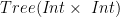. A consequence of changing the co-domain of is changing the domain of it to . We represent as . Now we can be more specific with our graphic:

function rec

Here we have to get a function that co-domain is . Probably the best is to pass the first part of the tuple (part with type ) and the rest (part with type ) is just a of the function . So, now our graphic is:

As you can see, the second part of the co-domain of is the type of function :

So our final graphic became:

Now, we just have to define the function and apply them to our anamorphism of .

h :: (Int, Int) -> ( (Int, Int), [ (Int, Int) ] )
h(0,0) = ( (0,0), [] )
h(v,0) = ( (v,0), [ (v-1,0) ] )
h(0,p) = ( (0,p) [ (0,p-1) ] )
h(v,p) = ( (v,p), [ (v-1,p), (v,p-1) ] )

And this is it! Now we can say that:
where

Outroduction

Here is all the code you need to run this example in Haskell:

module AnamorphismExample where

infix 5 ><

i1 = Left
i2 = Right
p1 = fst
p2 = snd

data Tree a = Node (a, [Tree a]) deriving Show

split :: (a -> b) -> (a -> c) -> a -> (b,c)
split f g x = (f x, g x)

(><) :: (a -> b) -> (c -> d) -> (a,c) -> (b,d)
f >< g = split (f . p1) (g . p2)

inTree :: (a, [Tree a]) -> Tree a
inTree = Node

anaTree h = inTree . (id >< map (anaTree h)) . h

-- our function
h_gen :: (Int, Int) -> ( (Int, Int), [ (Int, Int) ] )
h_gen(0,0) = ( (0,0), [] )
h_gen(v,0) = ( (v,0), [ (v-1,0) ] )
h_gen(0,p) = ( (0,p) , [ (0,p-1) ] )
h_gen(v,p) = ( (v,p), [ (v-1,p), (v,p-1) ] )

state = anaTree h_gen

Pass a year since I promised this post. The next will be on hylomorphisms I promise not take too that much.

Cryptol the language of cryptography

Pedro Pereira and I are working on a new project in the Masters. The second half of the Masters is composed of a single project suggested by a company. Some companies are forming partnerships in the Masters formal methods, including: the Critical software, SIG and Galois. We chose the Galois because we also are in the area of cryptography and we already knew some work of some people from this company.

The project suggested by Galois was study the Cryptol as a language of specification of cryptographic algorithms. The cipher we used for this study is the SNOW 3G (The SNOW website), later on I will talk about the specification of this cipher. In this post I am only interested to show the language.

I’m going to show you some details about the language. This post is not intend to be a exhaustive explanation of Cryptol, if you looking for that you can go directly to the manuals. This post only relates my experience, and what I like it most with the language.

Overview

Cryptol is a high-level language that is geared to deal with low-level problems. Is a Domain-specific language to design and implement cryptographic algorithms.
This language has a high percentage of correctness of the implementation of a cipher, because it implements type inference, so we can say that a big part of the language implements correctness. This correctness is also achieved thanks to the architecture of the language – functional. We don’t have side effects – a function only return something inside is codomain.
In Cryptol we have this philosophy that says that everything is a sequence. This is very useful because we are working with low level data (array of bits), so we use sequences to represent that arrays. We can have nested sequences to have a more structured representation of data. For example, we can simply transform a 32-bit sequence in a 4 1-byte sequence.
The size of this sequences could be implemented as finite or infinite, as we going to see later in this post. Because Cryptol is a high-level language we can also implement polymorphic functions, most of the primitive functions are implemented in polymorphic mode. The way we have to navigate throw the sequences is using recursion, or sequences comprehension, and with these two techniques we can implement recurrences.

If you are a Haskell programmer you just need the next section to learn Cryptol. This language is so look a like with Haskell that even the philosophy seems to have a lot in commune.

Types in Cryptol

The type means that you have a sequence of 32-bit size. All the types in Cryptol are size oriented. The unit is the , that you can use to represent . To represent a infinite sequence we use the reserved word , and we write: to represent that.

If you want to generate a infinite sequence, we use the syntactic sugar of the sequences like that: . Cryptol will infer this sequence as type

That means this sequence have infinite positions of 1-bit words. The type inference mechanism will always optimize the size that he needs, to represent the information.
So, it infer the type of as:

Because, it “knows” that needs only 7-bits to represent the decimal . But if you need more, you can force the type of your function.
We implement polymorphism in our types, if we have:

This means, that the function have polymorphism over , because we say that it domain is one sequence of size of type , and it codomain also. Here we could also see: meaning that is a constant of sequences of size of type , times.

So, lets talk about some primitive functions in Cryptol, and its types. The function have the following type in Cryptol:

As we can see, Cryptol is so size oriented, that we can use arithmetic operators in types. We can probably infer what this function does just from it type: works for all and such that if we have one sequence os size of type it returns one sequence of size of same type. In fact this function removes the first element of one sequence.

Because of this size oriented philosophy a lot of functions, that change the size of the sequences can be read just from the type.

As you can see in the following list of Cryptol primitive function:

Recursion and Recurrence

Cryptol implements Recursion, just like a lot of functional languages do.

Imagine the fibonacci function definition:

It implementation in Crytol is exactly the same as defined mathematically.

fib : [inf]32 -> [inf]32;
fib n = if n == 0 then 0 else if n == 1 then 1 else fib (n-1) + fib (n-2);

Cryptol uses recursion to permit us to iterate throw sequences.

But, If you prefer you can implement a more functional algorithm of fibonacci function in Cryptol:

fib : [inf]32 -> [inf]32;
fib n = fibs @ n;
   where {
      fibs : [inf]32;
      fibs = [0 1] # [| x + y || x <- drop (1,fibs) || y <- fibs |];
   };

Here, as you can see, we define a infinite list of all the fibonacci numbers, by calling the inside the sequences comprehension , this is called a recurrence, and you can use that too in Cryptol.

Cryptol vs C

I’m going to show you some part of the implementation of SNOW 3G in C. This is a function called

MULa : [8] -> [32];
MULa(c) = join ( reverse [
   ( MULxPOW(c, 23 :[32], 0xA9) )
   ( MULxPOW(c, 245:[32], 0xA9) )
   ( MULxPOW(c, 48 :[32], 0xA9) )
   ( MULxPOW(c, 239:[32], 0xA9) ) ] );

/* The function MUL alpha.
    Input c: 8-bit input.
    Output : 32-bit output.
    See section 3.4.2 for details.
 \*/
u32 MULalpha(u8 c) {
 return
  ((((u32)MULxPOW(c,23, 0xa9)) << 24 ) |
  (((u32)MULxPOW(c, 245,0xa9)) << 16 ) |
  (((u32)MULxPOW(c, 48,0xa9)) << 8 ) |
  (((u32)MULxPOW(c, 239,0xa9)))) ;
}

You can see that in Cryptol we just say that we want to work with a 32-bit word, and we don’t need to do any shift to our parts of the word. We just join them together. We reverse the sequence, because Cryptol stores words in little-endian, and we want to keep the definition like the specification.

This is a very simple function, so the result in C is not so that different. But if we have a more complex function, we were going to start having a nightmare to write that in C.

Conclusion

Well, the conclusion is that Cryptol is a language that really help to write low-level algorithms. With Cryptol the specification is formal and easier to read than other languages. A value of Cryptol is that the code can be converted to other languages, such as VHDL and C.

If you’re interested, take a look at the presentation that we did.

References

• Cryptol, the language of cryptography, now available
• SNOW wikipedia entry
• SNOW 3G Specification (pdf)
• SNOW site

Type inference

Intro

The type inference is the ability to a programming language deduct the data types of all functions of a program. It is a feature present in many strongly typed languages, such as Haskell. Where is not mandatory write the signature of the functions. What is great because it increases the production of code, and security because if the inference algorithm fail means that we have an error of types in our code, all this in compilation time.

As I said in previous post, one of the upgrades of Pointfree calculator is the type inference. After reading some scientific articles about Damas-Milner algorithm, also known as W algorithm, I began to imagine a way to implement this in Java, which is the mother language of Pointfree calculator. I started to do some sketches on paper and, after talking with professor José Nuno Oliveira, I realize that the algorithm isn’t that hard.

Remainings

Definition of (either in Haskell):

NOTE: in types means Either in Haskell

Definition of :

Type signature of Left and Right:

Talking same language

I will use a different notation to represent the domain and codomain of functions in order to help the explanation of the algorithm.

For function we have the type:

I will write that as:

Remember the definition of , we receive two functions, f and g. Because the notation is in pointfree, we represent also de domain and codomain of function in front of that, like we do for f and g.
In fact the type of is represented as:

I will also use the symbol , to say that type a unify with type b, that means, informally, that .

Let’s infer!

I will explain the algorithm to infer the type of function f:

The first step of the algorithm is attribute to all functions polymorphic types, so I will call the first type and the last

Because, have type , we conclude ;
Also, because have the type , we can conclude ;
Same thing to , that have the type , we can conclude and , so we have:

Because, the definition of : , we can say that the domain of f is equal to codomain of g, and so we can conclude , as we replace a type that is used in the codomain of first Right, we must also conclude , so:

As I explain before, the function , have the following type: , so:
and ;
Because have the type: , so and :

Because the definition of is , we need the same codomain in both functions, so we conclude , as both type trees have the same structure, we can conclude even more: , so:

And now we have the function, just with the needed types to simplify:

.

Now we just need to unify: and ,

.

We infer the type for function , .
Or if you prefer; in Haskell:

f :: Either (Either a b) c -> Either a (Either b c)